A Monte Carlo Algorithm for Computing pi

To illustrate running a job under Condor, you will use a Monte Carlo method for computing π

This is an example of an embarrassingly parallel problem that can easily be run on the Campus Condor Pool.

To illustrate running a job under Condor, you will use a Monte Carlo method for computing $\pi$ . This is an example of an embarrassingly parallel problem that can easily be run on the Campus Condor Pool.

Monte Carlo Algorithm

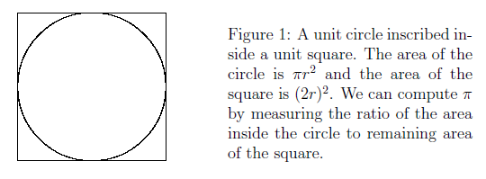
Consider the familiar example of finding the area of a circle. Figure~?? shows a circle of radius $r = 1$ inscribed within a square. The area of the circle is $A_s = \pi r^2 = \pi 1^2 = \pi$ , and the area of the square is $(2r)^2 = 2^2 = 4$ . The ratio of the area of the circle to the area of the square is:

$\begin{equation*} \rho = \frac{A_c}{A_s} = \frac{\pi r^2}{(2r)^2} = \frac{\pi}{4} \end{equation*}$

If we could compute the ratio $\rho$ , then we could multiple it by four to obtain the value of $\pi$ . One particularly simple way to do this is to pick regularly spaced lattice points in the square and count how many of them lie inside the circle. Suppose that we pick the points $(x_i, y_j)$ defined by:

$\begin{align*} x_i &= -1 + \frac{2i-1}{32}\quad i = 1, \ldots 32 \\ y_j &= -1 + \frac{2j-1}{32}\quad j = 1, \ldots 32 \end{align*}$

Then we find that there are $812$ points inside the circle and $212$ points outside the circle. The ratio is then $\rho = 812 / (812 + 212) = 0.79296875$ and so our estimate of $\pi$ is $\pi \approx 3.171875$ . This is obviously not a very good approximation.

Rather than picking a regularly spaced lattice, we can use Monte Carlo to compute $\pi$ . Monte Carlo methods can be thought of as statistical simulation methods that utilize a sequences of random numbers to perform the simulation. In a typical Monte Carlo process, we compute the number of points in a set $A$ that lie inside a region $R$ . The ratio of the number of points that fall inside $A$ to the total number of points tried is equal to the ratio of the two areas (or volume in three dimensions). The accuracy of the ratio $\rho$ depends on the number of points used, with more points leading to a more accurate value. Monte Carlo methods like this are a good way of computing the values of complicated higher-dimensional integrals.

A simple Monte Carlo simulation to approximate the value of $\pi$ is to randomly select points $(x_i,y_i), i= 1, \ldots n$ in the unit square and determine the ratio $\rho = m/n$ , where $m$ is number of points that satisfy $x_i^2 + y_i^2 \le 1$ .

Write a C program that computes $\pi$ using this Monte Carlo method. Your code should take two command line arguments: the first should specify an integer number of points to use in the Monte Carlo, and the second should be a string which specifies the name of a file that your program should write its output to. Your program should print out to the specified file (not to the screen) columns containing the number of points inside the circle $m$ , the total number of points $n$ , the ratio $\rho$ , the value of $\pi$ , and the absolute error in the value of $\pi$ . To compute the error, compare your computed value of $\pi$ to the C standard library value stored in the constant M_PI. You should use double precision numbers for these calculations and make sure that the columns in the file contain sufficient precision using the appropriate format statement in your fprintf.

To compute the random numbers that you will need in this Monte Carlo, you should use the C standard library functions rand() and srand(). A digital computer cannot generate truly random numbers unless it is connected to a physically random source, however the C library provides a way of generating pseudo-random numbers that will be sufficient for our purpose.

Random-number generation is a complex topic. The book Numerical Recipes in C provides an excellent discussion of practical random number generation issues in Chapter 7. For the this exercise, you can generate a random number between zero and one with the following code

x = (double) rand() / (double) RAND_MAX;

You will need to #include <stdlib.h> to use rand(). Type

man 3 rand

for more information on the function.

Pseudo random number generators need a seed to start the random number generation. If you do not specify a seed to rand() it will use the number 1 and generate the same sequence of “random” numbers each time. Sometimes this is desirable, but not in our Monte Carlo simulation. Before you call rand() for the first time, you should call srand() to seed the random number generator. srand() takes an integer as its only argument. A different integer will generate a different sequence of “random'” numbers.

There are a variety of ways to seed a pseudo random number. The best way is to read an integer from the system file /dev/urandom using the usual fopen(), fscanf(), and fclose() calls.

/dev/urandom is a special system file that looks at read-world entropy (time between keystrokes, packets on the network, etc.) to generate random data. If you cannot use /dev/urandom, then you can use the system call time(NULL) to return the time in seconds since 00:00:00 UTC, January 1, 1970. If you use time() you will need to #include <time.h>. Make sure your program uses one of these methods to seed the random number generator in your Monte Carlo code.

Use the time command to time how long your program takes to run for $n = 10^2, 10^3, 10^4, 10^5$ , and $10^6$ points (use the value of user time, which gives the amount of time your code spent on the CPU performing calculations). Make a plot that shows the error in your computed value of $\pi$ as a function of the number of points. Your report should state how quickly your code is converging on the value of $\pi$ (i.e. what is the order of convergence as a function of $n$ )? A log-log plot will make it easier to see this.

A Large-Scale Monte Carlo on Condor

Computing a very accurate value of $\pi$ in the way described above will take some time, as the convergence as a function of $n$ is quite slow. When we encounter a problem such as this, high throughput computing is a good way of solving the computational bottleneck.

First recompile your Monte Carlo code, but add the commands -static and -static-libgcc to your compile line. For example, if your program is called computepi.c then you should compile it with

gcc -static -static-libgcc -Wall -o computepi computepi.c -lm

This makes your code more portable for running on the campus Condor pool. Check that this worked by running the command dd on your executable. If it prints

not a dynamic executable

then your code compile correctly. If it prints something like
linux-vdso.so.1 => (0x00007fff8edff000)
libc.so.6 => /lib64/libc.so.6 (0x00000038cba00000)
/lib64/ld-linux-x86-64.so.2 (0x00000038cb600000)

then you need to re-compile with the static options. Use scp to copy your executable from

phy607.phy.syr.edu to its-condor-submit.syr.edu

Write a Condor submit file that executes your program on the Campus condor pool for $n = 100$ points. To specify an argument to your program, you need to add the line with the \verb|arguments| keyword in your submit file. For example, to run the program computepi with 100 points and write to the file pi_output.txt, the Condor submit file would begin

universe = vanilla
executable = computepi
arguments = 100 pi_output.txt

Don’t forget you need the rest of the submit file described previously to get your job to run. I suggest copying and modifying hello.sub for this purpose. Submit this job and check that it works. If you are having trouble running a Condor job, see me.

Using your timing data from the previous exercise, estimate how many points $n$ it would take for your program to execute for approximately two hours. Modify the arguments line in your Condor submit file to use this value of $n$ . To parallelize the task, use the queue line in your submit file to submit 1000 jobs to the pool. We now have a problem: if all of your jobs write to the file output.txt they will overwrite each others results.

Fortunately, we can use the Condor $(cluster) and$ (process) variables to ensure that each job writes to a different file. To do this, your Condor submit file should read

arguments = 100 pi_output. $(cluster).$ (process).out

Once you have done this, submit the jobs to the Condor pool. This may take some time to run, so leave yourself plenty of time to do this.

Write a second program that reads in the values of $m$ and $n$ from the output files of computepi and used all of the measures values to compute $\pi$ . How accurate is your value now? Add a point to your graph showing the accuracy as a function of $n$ . Is it consistent with your predictions? How long would it take you to compute $\pi$ to an accuracy of $10^{-4}$ , $10^{-6}$ and $10^{-15}$ using this method?

Your report should include all your C code and your Condor submit files.

Monte Carlo Algorithm Link

A Large-Scale Monte Carlo on Condor Link

Monte Carlo Algorithm

A Large-Scale Monte Carlo on Condor